@marcob, @ntjahj, @eilah_tan, @sandrapalka let’s use this thread as a shared notebook for stuff we find out.
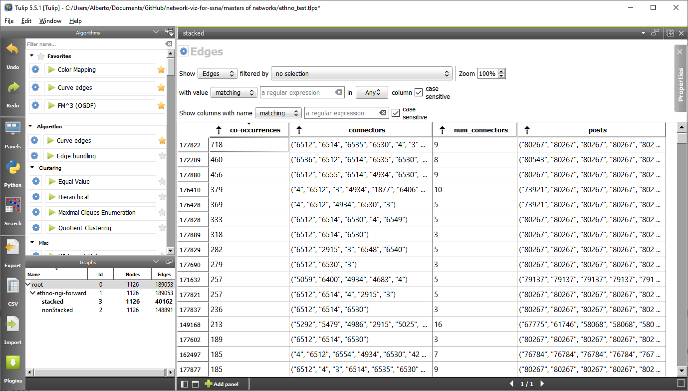
As requested by Natalie, I added some code in my scripts so that now you can see the post IDs behind each edge. Now the spreadsheet view of the stacked graph looks like this:
-
co-occurrencesmeans in how many different posts the connection between the two codes connected by this edge occurs. -
connectorsis the list of user_ids of the people that authored those posts.
*num_connectorsis the number of those people. It can never be larger thanco-occurrences. -
postsis the list of post_ids that were coded by the ethnographer with both those codes.
To see a post on Edgeryders, go to https://edgeryders.eu/posts/post_id.json and look for the field “raw”. This is Use Firefox, which will display the post in a nice way:

There is also another way, but the code has been a bit abandoned, so I don’t trust it completely.
https://graphryder.edgeryders.eu/ngi
Go to “Code view Full”, then select the interactor that looks like an eye and click on the edge. A list of posts should open.
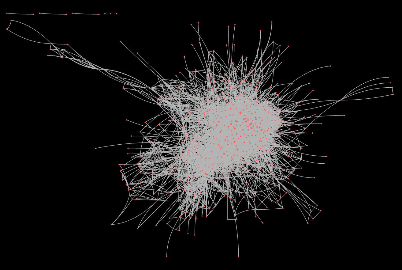
Besides giving support to other people in the group wishing to explore the data, I have been working on an interpretable, theoretically justified way to filter it. First of all, SSNA corpora are quite large. NGI Forward’s codes co-occurrence network has (at the moment) 1,120 ethno codes, connected by 148K co-occurrence edges.
Interpretation of the high connectedness of these networks. A single longish and rich post might be associated with as many as 30-50 codes. By construction, a post coded with n codes gives rise to a n - clique of co-occurrence edges: each code co-occurs with all the others. The single post adds
n(n- 1)/2edges.
Recall that we interpret co-occurrence as association.
Interpretation of co-occurrence as association. If two codes co-occur, it means that someone has made references to the concepts or entities described by the codes in the same utterance. Hence, this person thinks there is an association between the two.
So, which are the strongest associations? Two simple ways to think about this:
- The ones with the highest number of co-occurrences (call it k) are the strongest. This is the one we have been using so far.
- The ones backed by the highest number of individual informants (call itk_p) are the strongest.
Both ways require the construction of a new network, where edges representing single co-occurrences might be “stacked” on top of each other, to represent in one single edge all the associations made in the corpus between the two codes.
Interpretation of an edge in the stacked graph. In the stacked graph, any two nodes can be disconnected or connected by one single edge. If they are connected, that edge represents all the associations made in the corpus between those two edges.
Interpretation of k. k is a measure of intensity of the association between two codes. The higher it is, the richer the context in which the association is made.
Interpretation of k_p. k_p is a measure of the breadth of agreement about the fact of the two codes being associated. The higher it is, the more numerous are the informants that make that association.
These two measures have opposite shortcomings. k does not account for numbers of people making the association. In the limit, a single informant could drive high levels of k if she or he keeps bringing it up in many different contributions to the corpus. Relying only on k might mean giving excessive attention to vocal minorities, obsessively going on about their favourite subjects.
k_p does not account for depth of reflection. A mention dropped casually, once only, by one informant, has the same effect on k_p as any number of thoughtful, well explained and documented contributions by someone with deep expertise. Relying only on k_p might mean rewarding shallowness over depth.
Both indicators assume a special meaning when they are equal to 1.
When k = 1, the two codes only co-occurred once. It could have been a random event. At any rate, a single co-occurrence does not meet reasonable criteria for collective intelligence. All edges with k = 1 should be discarded when studying the codes co-occurrences network.
When k_p = 1, the two codes may have co-occurred more than once, but always in contributions made by the same single informant. It could be an idiosyncrasy of that person. At any rate, the co-occurrence reflects one single opinion, and, again, it does not meet reasonable criteria for collective intelligence. All edges with k_p = 1 should be discarded when studying the codes co-occurrences network.
Note that, for each edge e, k(e) >= k_p(e). So, discarding edges where k_p = 1 will automatically get rid of all edges where k = 1. When I do this on the NGI Forward co-occurrence network, I get a reduced network.
| nodes | edges | |
|---|---|---|
| non-stacked network | 1,120 | 148,565 |
| stacked network | 1,120 | 39,942 |
| k_p > 1 | 544 | 5,912 |
The reduced network is still much too large to process.
From now on, we have to make more arbitrary choices. I propose to use k_p as a filter, and k as an indicator of quality. A natural-language algorithm for building a reduced network could look like this:
- Decide what is your minimum accepted level of breadth of agreement on an association (k_p) for you to take it into consideration. We already know this level should be at least 2, but it could also be higher. Only include in your network the edges that meet this minimum accepted level.
2. Now include in your reduced network the highest-k edges that meet this requirement. Lower k, and repeat. Keep lowering as long as your reduced network stays readable, then stop.
So, intensity of association is the main measure of edge importance, but if a minimum width of agreement is achieved.
How much information do we lose as we do so? I have several ideas in this direction, I will continue to explore them tomorrow.
How much information do we lose when we filter in only edges whose k_p value is above a minimum threshold?
Let’s make a few observations based on the NGI Forward dataset.
-
k and k_p are positively correlated, but not as tightly as you might think (0.41).
-
There are quite a lot of edges with high k, but a relatively low k_p. As a result, when we impose a higher k_p threshold, even by just one unit, we are throwing away many high-intensity edges. Let us consider only the values of k_p between 2, the minimum, and 6:
Codes Edges k <= 5 k from 6 to 10 k from 11 to 20 k from 21 to 50 k > 51 kp >= 2 544 5912 3087 1434 831 426 134 kp >= 3 289 1574 380 484 395 221 94 kp >= 4 170 512 34 145 159 117 57 kp >= 5 89 168 2 29 48 47 42 kp >= 6 47 74 0 7 16 26 25 We start from the theoretically justified minimum value of k_p, 2, and move up from there to 3. Compare lines 2 and 3 of the table above: as we do so, we get rid of 3,087 - 380 = 2,707 edges with k <= 5, which is what we want. But we also lose 1,434 - 484 = 950 edges with k between 6 and 20, 831 - 395 = 436 edges with k between 11 and 20, 205 with k between 21 and 50, and even 134 - 94 = 40 edges with over 50 co-occurrences.
Faced with substantial loss of high-intensity edges, the ethnographer might be tempted to use a double criterion for edge inclusion: for example, she could include edges with either a minimum value of k_p (for example 4, which reduces this dataset to manageable proportion) or a minimum value of k (for example 50). This is more flexible, but also more ad hoc.
I did a supplement of analysis inspired by some remarks by @amelia. My original question to her:
Consider two edges e1 and e2 in the codes co-occurrence network. They both have the same values of k (number of posts in which they co-occur) and k_p (number of people who authored the same posts). The posts in e1 are concentrated in one or a few topics, whereas those in e2 are more spread out.
- Is this difference relevant to a qualitative analyst?
- If so, in what sense? Is it “one single topic is great, deep conversation makes for better alignment”, or is it “more topics are great, it means there is more stability in this association”?
Amelia’s reply what that these two metrics have different meanings:
they are both great – but for different reasons.
for the former, you’d need more “cases” to be able to say whether or not the themes that come up in it are shared across different people/places (framing depends on what it is, ofc)
but you’d know that that thread would give you a lot of places to start in terms of questioning a larger group
you’d get a deeper sense of what the key problems/analytics are
in the latter, i’d say – ok I now know that these two topics together are definitely an association worht querying
and now I have to say, how do i dig deeper to understand the dynamics of that association
So I set out to explore that relationship. We are now left with three metrics:
- Number of posts on which the co-occurrence is made. We call it k
- Number of people who authored those posts. We call it k_p, or kp in short.
- Number of topics or threads on the forum on which those posts appear. Let’s call it kt.
The mathematical relationships governing them are such that, for any edge e:
k(e) >= kp(e)
k(e) >= kt(e)
There is no special mathematical relationship between kp and kt. However, we do have a very strong statistical correlation between the two. In this next table, I show the Pearson correlation coefficients between k, kp and kt in the three SSNA datasets considered.
|||k|kp|kt|
| — | — | — | — | — | —|
| ngi forward|k|1.000000|||
| |kp|0.417991|1.000000||
| |kt|0.313440|0.886162|1.000000|
|opencare|k|1.000000 | | |
| |kp|0.551894|1.000000| |
| |kt|0.548064|0.884673|1.000000|
|poprebel|k|1.000000| | |
| |kp|0.240738|1.000000| |
| |kt|0.203754|0.944228|1.000000|
Despite some diversity in the coding style and degree of interaction across informants, the three datasets display a remarkably stable behaviour. The correlation between kp and kt is very strong, hovering around 0.9. On the other hand, k is still positively, but more weakly, correlated with both kp and kp, with coefficients ranging between 0.25 and 0.55.
My provisional conclusion is that it is probably not worth it tracking separately kp and kt, as they bring in very similar measures of diversity. Network reduction based on those measures are unlikely to yield very different reduced networks.
kp is more intuitive and easy to interpret, so I would suggest we use that over kp.