This topic is a linked part of a larger work: “Edgeryders OÜ Company Manual”
For budgeting in Edgeryders’ projects, we developed an open source spreadsheet called “Budget Template v3”. This is its documentation. It works in tandem with another spreadsheet “Magic Spreadsheet v1”, used for company-wide cashflow management and documented here.
If you want to use these tools in your own organization, get them here.
Content
1. Budget tasks before a project
- 1.1. Getting the budget spreadsheet
- 1.3. Starting a budget spreadsheet
- 1.3. Sending a proposed budget to the client
2. Budget tasks during a project
- 2.1. Updating the cash flow projection with accounting numbers
- 2.2. Monitoring the project’s cash flow
- 2.3. Managing forex conversions
- 2.4. Tracking internal budget shuffling
3. Budget tasks after a project
1. Budget tasks before a project
1.1. Getting the budget spreadsheet
We have published our spreadsheet under an open source licence, so you can use it in your own organization. Instructions for getting and installing it are in Github repo edgeryders/magic-spreadsheets.
As a demo and to follow the instructions below, we also provide a public demo version of the Budget Template v3 spreadsheet.
1.2. Starting a budget spreadsheet
-
Find a placeholder spreadsheet to use. In the Edgeryders organization, we always have a few placeholder budget spreadsheet files around – just take one and use it for your project. It is already pre-registered in our Magic Spreadsheet (which aggregates project budget information).
Simply go to Edgeryers’ Google Drive Enterprise and into folder “Team Drives → All Teams Drive → Templates”. There, find a spreadsheet named “Budget Template v3: Placeholder Project …”. That’s the one to take . There should usually be two variants: those with “(EUR only)” in the filename, and those without. If your project is budgeted and paid in EUR, preferably use one of the “(EUR only)” ones, as it saves you some of the more complex steps below.
(As a project manager, you should have read / write access to that folder – if not, ask @matthias or another one who has. And if no placeholder budget spreadsheet of the type you need is left, ask @matthias to make more, or check at the end of this manual to see if you want to do it yourself.)
-
Rename your spreadsheet file. This prevents anyone else from taking it for their own project.
-
Move your spreadsheet file into the Team Drive and folder that you use for your project.
-
Fill in the basic project info. This goes into your copy of sheet “Overview”. Only fill in the yellow fields – everything else will be calculated automatically. Hints:
-
Help messages. You will find help messages when mousing over cells with a note, indicated by a small black triangle in the top right.
-
Adding team members. You can add any number of team members so that they become available in the “Cost” sheet, column “C (Person)”. For that, simply insert new rows between the existing “Team” rows. That automatically enlarges the named range needed for the dropdown on the “Cost” sheet as well. Just filling empty rows at the end of the sheet does not.
-
-
Remove the second currency (if applicable). The budget template was made to suit projects with a non-EUR primary currency, in a way that allows us to use EUR internally and to avoid any forex risks. If your project budget is in EUR already, you don’t need that feature. If you did not already start with a placeholder spreadsheet that had it removed, you can remove it as follows. You could also use the spreadsheet without removing columns, but then you have always a redundant column around as both currencies are “EUR”.
In the instructions below, column and row identifiers always refer to the state when you get to that step: after deleting a column G, there will be a new column now labeled G and a succeeding step may refer to that.
-
In the Cost sheet, delete column G (“Unit cost: EUR”).
-
Unmerge cell G1 (select it, then “Format → Merge cells → Unmerge”).
-
Copy column G (“Budget: [primary currency]”) over column H (“Budget: EUR”).
-
Delete column G (“Budget: [primary currency]”).
-
In the Revenue sheet, unmerge cell D1.
-
Copy column D (“Revenue: [primary currency]”) over column E (“Revenue: EUR”).
-
Delete column D (“Revenue: [primary currency]”).
-
In sheet “Overview”, repair the formula for “Project profit” (cell B6). It should now be
=Cost!$G$nn / $B$14, withnnreplaced with the number of the last filled row on sheet cost – the one for “Edgeryders margin”. -
In sheet “CashflowData”, adapt the formula in cell A4 to use columns
A, C, Dinstead ofA, C, E. So the formula would then be:=QUERY(RevenueData, "SELECT '"&ProjectName&"', '"&Status&"', A, C, D LABEL '"&ProjectName&"' '', '"&Status&"' ''" )
-
-
Make the first status log entry. Go to sheet “Status”. There are some example rows that you’ll have to delete, while adapting the first one to your case. Afterwards, it will look like this:
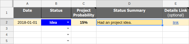
It is important to keep this up to date, esp. to set the “Status” column to “Active” after a contract was signed. Because only projects marked “Active” are included in the company-wide cashflow prediction in our Magic Spreadsheet. Also, the project probability numbers will be used to estimate the worth of Edgeryders’ project pipeline.
-
Fill in the revenue items. Adapt sheet “Revenue” so it reflects the dates and amounts of the invoices you expect the client to pay, according to the contract conditions.
-
Deleting rows. You can delete any of the example rows without issues. When deleting an own row, remember to also delete the corresponding column in the Revenue sheet.
-
Adding rows. You can add a row at any location and fill it with a copy of an existing row.
-
-
Fill in the cost items. Adapt sheet “Cost”. Each line represents one budget item or sub-item, and a billing plan structured by the receipt of client money. The billing plans are then summarized into a tabular cash flow plan in row 5 (“Cash on hand”).
-
Deleting “Cash flow” columns (J-N). All except the last column can be deleted. The last one calculates the remainder of the budget item to be billed at the end of the project, and should not be deleted. (If this is the only remaining one, you will also have to adapt the formula to calculate its cells to fix the
#REF!error that you’ll see.) The number of columns must match the number of revenue items in your Revenue sheet. -
Inserting new “Cash flow” columns (J-N). Insert columns only between two existing cash flow columns, as that will automatically update the ranges in formulas as needed. After that, fill the column header (rows 2-5) with a copy of that of any existing cash flow column except the last one (because that one has a conditional formatting assigned to warn when projects make <20% profit). The number of columns must match the number of revenue items in your Revenue sheet.
-
Deleting cost (sub)item rows. You can delete any row without issues, except the last one containing the Edgeryders margin (because it contains different formulas that you’d have to get back from the spreadsheet template if you accidentally delete this line and want it back later). If you delete a budget item row, also delete all its subitem rows, if any.
-
Inserting a new cost item row. Only insert new rows between existing budget rows, (below the first one or above the last one) as that will automatically update the ranges in formulas as needed. Then fill the row(s) with a copy of an existing budget item (or item incl. sub-items, as needed) to prime it with the correct formulas. Adapt the cell contents as needed.
-
Inserting a new cost subitem row. Only insert new rows between subsequent budget subitem rows, as that will automatically update the ranges in formulas as needed. Then fill the row with a copy of an existing budget subitem to prime it with the correct formulas. Adapt the cell contents as needed.
-
Adding cost items. To add cost items, first decide how many units of that item you are going to pay for, and how much each units costs. For example, if the item concerns contracting Alice for 2 months of full-time equivalent work on this project, write
Alice's workin column B; chooseAlicefrom the drop-down menu in column C; write2in column D; writeFTEin column D. Column F contains the cost of one unit of the item: in this case, suppose that Alice’s monthly full time equivalent cost is 5,000 EUR, you enter5000in column F. -
Allocating costs to invoices. A key design element of our budgets (and of our finances themselves) is that each cost item is allocated to a revenue item. This helps us enforce the principle of cash flow positivity. In the
Costtab of the budget template, each column markedCash flowcorresponds to one revenue item. (You entered revenue items in theRevenuetab, see above.) The cells in those columns come pre-filled with a formula; change that as appropriate, using either formulas or absolute numbers. Do not change the rightmostCash flowcolumn: it automatically assigns to the final revenue item all costs that have not been assigned to any previous revenue item. If you need more or less revenue items, add or remove columns according to teh instructions above for deleting / inserting “Cash flow” columns. -
Using custom formulas. You can use a custom formula in a cell without issues. Most likely you’d use one in the Cost sheet, in the “Quantity” or “Unit cost” columns. If you use a formula, always explain in a note what it means so that your budget spreadsheet stays legible for others. For example: when entering a formula “
=3.5*25%” into the “Quantity” column, add a note to the cell saying “”=3.5 months project runtime * 25% job".
-
Dealing with revenueless (investment) projects. Some projects have no revenue. These are the special “core” project, keeping track of fixed costs like the accountant and rent, and occasional investments we might make in business development. In this case, we recommend accounting for costs on a monthly basis. To do it, first create in the Revenue tab one revenue item per month that your project lasts; set each payment date in column C to the beginning of a month; and assign an amount of 0 to each item in column D. Then, proceed assigning costs to revenue items as normal. Since revenue items have a date, this allows us to know when we are going to incur these costs, and so to make reliable cash flow predictions.

1.3. Sending a proposed budget to the client
It’s probably best to create a copy of the whole file, or of the sheet in another tab, and adapt it by eliminating unnecessary / non-public information and adding client-facing information. And then to send a PDF export of that sheet only.
2. Budget tasks during a project
2.1. Updating the cash flow projection with accounting numbers
You can update the cash flow projection with numbers from our accounting system to “ground the projection in reality” at any time, but ideally after receiving an invoice from the client and before paying any project expenses after that:
-
In your Revenue sheet, enter the money you actually received from the client in the new invoice payment. If the project uses two currencies, enter the amount of EUR you received into the EUR column, replacing the automatic conversion from the primary currency.
-
In your Cost sheet, put the current total of project costs as shown in FreeAgent into the field for the sum of costs beneath the previous invoice you received, replacing the sum formula. Also set all cost sums for invoices before that one to zero. This way, when the formulas sum up all costs, it yields the correct results. (A bit more effort but tidier: instead of setting all previous costs sums to zero, leave them as they are and only enter the additional costs – not the new total – that accumulated since last updating from FreeAgent.)
-
If some collaborators did not yet invoice what they were allowed to in the now completed steps of the cash flow plan, move these positions to the current step of the cash flow plan. Otherwise, the sum of actual costs that you copied over from FreeAgent does not represent the reality of what is listed below it.
TODO: This process is a bit tedious. Also, it is only an approximation when using it at other times than immediately after an invoice was paid, as it does not know then which expenses have or have not been made in practice. Somebody should make it better ![]()
2.2. Monitoring the project’s cash flow
-
Update the cash flow projection with the latest numbers from FreeAgent, as instructed above.
-
Look at the cash flow projection in sheet “Cost”, row 5. Your current step in that cashflow plan is the column for the most recent invoice that has been paid.
In that column, row 5 shows how much cash you will have on hand after paying all expenses that are due between now and the receipt of the next invoice. In other words, all invoices up to and including the most recently received one are your budget to cope with until you receive the next invoice, and “cash on hand” is the remainder of that budget you’ll have when that next invoice comes in.
-
If this “Cash on hand” value for the last received invoice, or for any invoice after it, is negative: adapt the cash flow plan in consensus with your suppliers to make these “Cash on hand” values positive. We require all projects (except our internal investment projects) to be cash flow self-contained. If it is not possible in your case, apply to the management board for an exception.
2.3. Managing forex conversions
In projects that use a primary currency (for the contract and budget) that is not Euro, foreign exchange conversion is needed – because our accounting currency is Euro. By using the instructions below, it is possible to create contracts with all collaborators using Euros while still avoiding foreign exchange rate risks.
Making a contract. When making a contract with a collaborator, (1) make in for a payment in Euros, (2) put in the amount in Euros as shown by the budget template with the date of the contract as the forex conversion date in Overview!B8 and (3) note in the contract that the agreed-on total payment will be adjusted by the change in the conversion rate from the primary currency to Euros, between making the contract and the mid of the project. Such a rule is legally permissible because we work with independent contractors and not with employees.
Updating the forex conversion date. This date is entered in cell Overview!B8 and used to determine the forex conversion rate to use. At first, enter the date when the budget was created. When the project starts, update it sporadically to the current date until reaching a date in the center (or even better: “weighted center”) of the revenue payments. This will approximately calculate the average exchange rate of the money we receive from the client, and hand that down to collaborators.
Billing Edgeryders. For this, the project manager first has to share the project’s budget spreadsheet with view-only access rights with all collaborators mentioned in it. When the time comes to write a bill, the collaborator must take care to not exceed the allowable aggregate amount to invoice, as aggregated from the first to the current phase of the cash flow plan (hint ![]() ). This limit changes dynamically with the exchange rate, so has to be looked up shortly before writing the invoice.
). This limit changes dynamically with the exchange rate, so has to be looked up shortly before writing the invoice.
[TODO: Improve this whole mechanism and its documentation.]
2.4. Tracking internal budget shuffling
In many projects, the project budget total is fixed after client approval resp. receiving the grant. But within certain limits, you can still reshuffle the allocated money between budget positions internally, as long as the total does not increase.
To keep an overview of who introduced which changes when and why and how much budget remains unallocated internally, you can use the following technique:
-
On sheet “Cost”, create a new column
Hnamed “Allocation”. -
For each budget item, add zero or more sub-items to express what the budget is actually used for. (Remember to indent sub-items by four spaces more to get the right cell background shading.)
-
Fill columns “Item” and “Allocation” for these sub-items, not “Budget”. Optionally you can also fill “Person”, “Qty”, “Unit”, “Unit cost”, calculating “Allocation” from these.
-
Sum up the sub-items in the row of their parent item using a number rendered as gray text, for example
=TO_TEXT(SUM(H9:H5)). You can see this technique in the “Budget” column as well. Then sum up the whole “Allocation” column in the column header, making it easy to see when too much money is allocated internally. -
Fill column “Note” for these sub-items. Here, provide a journal of the changes to this sub-item. To preserve the journal, you would also not delete such a row but rather set its “Allocation” value to
0and add a journal entry about the change.In the journal, use a convention for formatting. We propose to use one line per change, in ascending order, with a line header in bold. With the cursor in the cell, in Google Sheets you can create a newline by Ctrl + Return an bold print by selecting text and pressing Ctrl + B. To keep the budget spreadsheet visually well navigable, set the row height to a single line of text manually. To read the journal text, one will then have to place the cursor into the respective field. An example value might look like this:
2019-09-01 by Matthias: Allocating the budget for 30% of my work here to my new assistant server admin.
2019-09-20 by Matthias: Allocating the budget for a total of 50% of my work here to the assistant. I like that help
This technique does not change the official budget approved by the client, but instead tracks the internal usage of these budget items in separate columns. These columns have informational character only and what is entered here is not used, for example, for company-wide cashflow monitoring. Because these numbers will sum up to at most the client-approved budget, which is the “worst case” then and already used for monitoring and reporting.
For an example of this technique in action, see our “NGI Forward Magic Budget” spreadsheet (if you can access it, of course).
3. Budget tasks after a project
3.1. Evaluating the project’s financial performance
-
Update the invoice amounts and costs one last time from FreeAgent once all invoices are in and all costs are paid. See for that section “Updating the cash flow projection with accounting numbers”.
-
Look at the project profit value in the Overview sheet.
-
If the project profit is less than 20%, look at the other sheets to find out why. As the project manager, report your results in the next project coordination / cash flow monitoring call. For that, see section “Monitoring the company’s cashflow” in our company manual.
[TODO: More details, better process.]
4. Admin tasks
4.1. Creating placeholder spreadsheets
Note that in almost all cases, you can just use an existing placeholder spreadsheet for your project. Only if we did run out of prepared ones, there is a need to create more, as detailed below. Usually @matthias will care for this and you should just tell him about this (except you want to try it yourself, in which case read on).
-
Create copies of spreadsheet “Budget Template v3”, in the same folder.
-
Name the copies
Budget Template v3: Placeholder Project [number], with a number that is in sequence with the last existing such file, or otherwise starts from 1. -
Adapt the project name in the spreadsheet. Make it also “Placeholder Project [number]”, consistent with the file name, by editing cell B2 in its Overview sheet.
-
Copy the URL of each placeholder spreadsheet into the Magic Spreadsheet for Edgeryders OÜ in sheet Projects, at end of column A.
-
Fill down column B in the Magic Spreadsheet in sheet Projects. The goal is that the
=IMPORTRANGE($A…, "ProjectData!A4:G4")formula already in use for the existing rows on that sheet is also used for the the new row(s) you just added to this sheet. -
Grant access. After finishing the preceding step, you will now see a
#REF!appear in the “Project Name” column. Mouse over it and click on the “Authorize” button that appears. This permanently allows the Magic Spreadsheet to access the placeholder spreadsheet (as long as you have access to the placeholder spreadsheet). -
Add an
IMPORTRANGE()statement for each new placeholder spreadsheet to the formula in the Magic Spreadsheet, sheet CashflowData1, cell A4.(This step is unfortunately necessary because
IMPORTRANGE()cannot be used as an array formula. We might use Google App Script, but that’s very proprietary so who wants to learn such a thing.) -
Fill the column for each new placeholder spreadsheet in the Magic Spreadsheet, sheet CashflowData2. There will already be a column with the project’s name at the top. Fill these columns with the right formulas by selecting the cells in the previous column (starting from row 6) and filling to the right to cover the new columns.
-
Remove the secondary currency feature from some spreadsheets. See section “1.1. Starting a budget spreadsheet” above, under point “Remove the second currency (if applicable).”. Do this for about half the placeholder spreadsheets you created, and mark them accordingly by appending " (EUR only)" to their filename and project name.
5. Design rationale
No accounting. We kept this budget spreadsheet purely as a planning tool – no backfeeding from accounting tools is needed beyond sporadic updates of paid invoices and aggregate expenses to serve as baseline for cash flow planning. The main advantage is that it avoids form filling work; the main disadvantage, that it cannot serve as a quick overview for project managers seeking to decide if a new bill can be approved or not. In addition, cash flow projections are approximate except when based on accounting numbers at the receipt date of a new invoice to the client. There is an earlier version (Budget Template v2) that solves these issues, but requires more form filling. You can create a budget spreadsheet on that basis, but might have to invest some work to iron out some remaining issues.
Prepare for adding and removing rows and columns. To make adding and removing data rows and columns simple, removing rows should not leave any invalid references. Formulas have been adapted accordingly, for example deriving the invoice serial number from the row number instead of “previous invoice number + 1”. That is also the reason for the strange formulas in the header of the cash flow plan columns on the Cost sheet: they calculate “sum of invoices up to this step minus sum of costs up to this step”, and because this formula is the same for all columns removing and adding columns presents no issue.
List of hacks. Some tricks had to be used to make everything work, so we better document them to keep the spreadsheet maintainable:
-
Suppressing
#N/AwithSUMIF(). This technique is documented here and applied in the Magic Spreadsheet inCashflowData2!D6:. -
Excluding cells from sums by using text. On the Cost sheet, there is a budget and cash flow plan for both a budget items and its subitems. But only one or the other must be included when calculating column totals, so the subtotals for the budget item are text cells rather than numbers. This way, they do not have any effect on column sums. All such text cells are shown automatically in gray to indicate that they are “inactive”, not making it into the sums.
-
Pretty-printing formulas. This requires to work around a bug in Google Sheets, and is documented here.