Recent techniques in neural networks applied to text analysis show very interesting results. Word2Vec captures, from a corpus of text, the semantic representation of a word in a space made of the other words composing the text. It is actually a bit more sophisticated but in the end, every word has a representation in an n-dimensional space, and close words that tend to appear often together in the corpus are supposedly placed close together in this high dimensional space. This allows for a word to be associated with its nearest neighbors in the high dimensional space, forming a sort of semantic vector representative of the word. This embedding allows vector comparison, such as, in a large Wikipedia corpus, the vector that differentiates Paris from France, should correspond to Berlin if placed from Germany. In that sense, the context from which you train your network has a strong impact on the semantic representation of the word. For example, football trained on a British corpus should refer to other vocabulary related to the sport known as soccer (such as corner, goalkeeper, and champions league) but trained on an American corpus, we would have a different contextual vector (such as quarterback, drop kick, or super bowl).
We launched only a small exploratory experiment to see how we could apply this technique to investigate the Opencare conversations. Due to the many languages, typos, etc., this experiment highlights the heavy requirement for advanced NLP pre-processing to improve the results. Then after training the network, we can explore a few queries, to see the representation network. The interesting insight would then be to find unexpected word association. The last step of our experiment is to construct the network of nearest neighbors words and see how communities/paths would form.
Requirements
Download and compile
https://code.google.com/p/word2vec/
You can copy the content of https://github.com/opencarecc/Masters-of-Networks-5/tree/master/word2vec into the word2vec folder you just created.
Details
- word2vec/scripts: scripts to run different steps
- word2vec/data: processing data
- word2vec/graphs: Tulip graphs (ready to run)
- word2vec/images: Images for this post
The input data
The raw Edgeryders’ OpenCare conversations: data/mon5.bcp
Preprocessing
Quick and dirty tricks to produce a ready-to-process dataset: scripts/clean_mon.py
- Removes web addresses and HTML code
- Corrects capitalization: aWordWithCapitalizationIssue -> a Word With Capitalization Issu
- Removes non-letter characters (actually it also removes accents etc.)
- Removes English stopwords and words of length <= 3 letters
- Lowercases the words for better comparison
- Stems the words (to extract roots for plural and conjugated form removal), with the Porter Stemmer, and use the most occurring form as representative of the class:
- learn -> learn (2)
- learning -> learn (10)
- learnt -> learn (5)
- → uses learning for all instances of learn, learnt, learning
- Create classes of words with very close Levenshtein distance (remove some letter inversion misspelling) -- currently deactivated due to possible delicate confusion (e.g. association of controversial and uncontroversial)
Ideally, we need to use a spell checker like pyenchant, and check the language first to find the right dictionary to use etc
- Finally we oversample the text a 100 times because the dataset is too small.
- The output data is a big text stored in data/mon5.cln
Neural Network
Train the network: scripts/word2vec_train_mon.sh
We threshold the min word occurrence to 101, due to oversampling
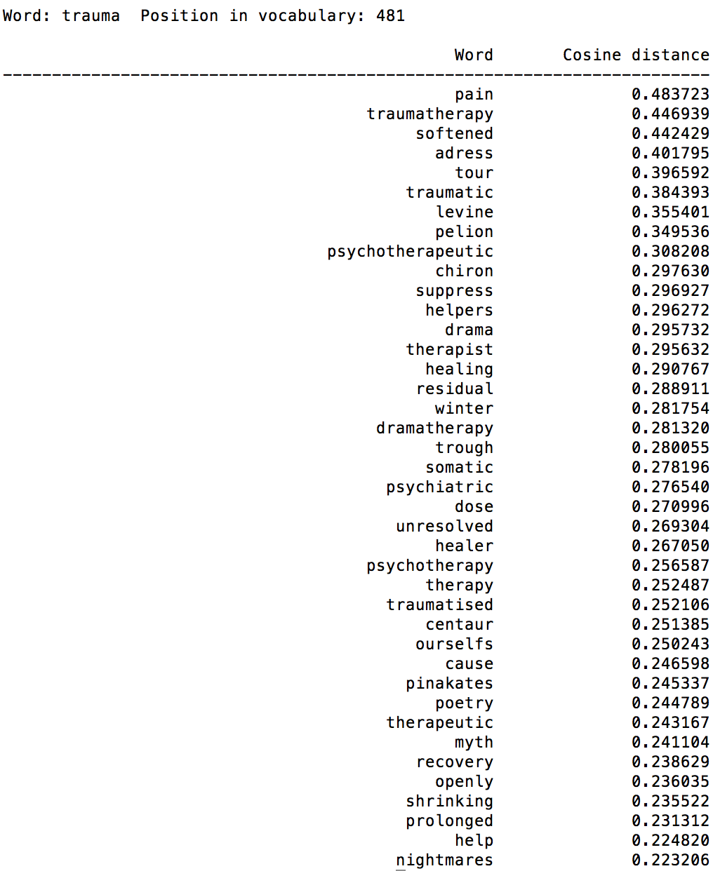
A few example queries:
|
|
|
|
|
|
|
|
|


Bonus: the file script/demo-analogy.sh allows to try testing analogies (such as Paris->France = x->Germany, x=Berlin). (need to find good examples!)
Word graphs
Constructing K-Nearest Neighbors networks
- A K-Nearest Neighbors (or KNN) graph connects words with their k- closest words (based on their cosine distance).
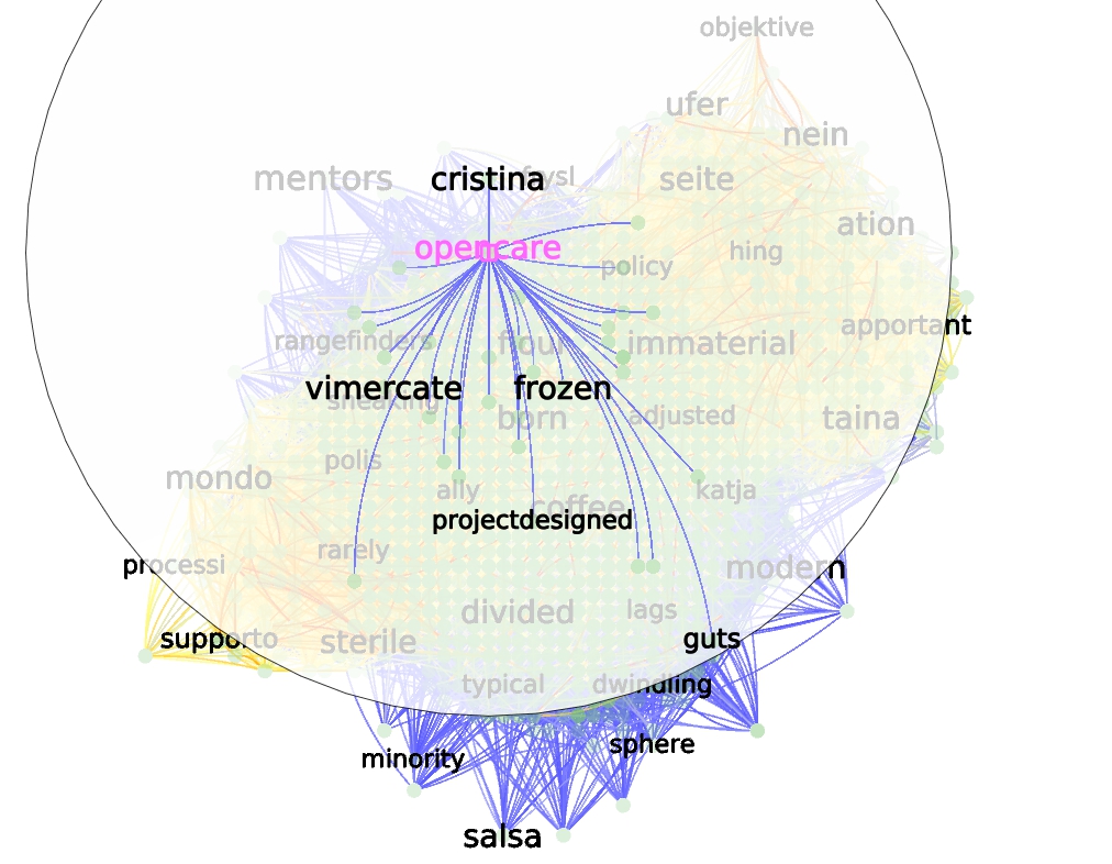
- The exploration of the vector space starts with the word opencare, then grows to the K nearest neighbors, then retrieve the K neighbors of these neighbors until no new neighbor can be retrieved.
- Edges are directed (same logic as the “best friends”: Thomas could be the closest neighbor to Georges, but Georges could have even closer neighbors than Thomas). Interesting relationships can then emerge from the mutual KNN, e.g. reciprocal relationships only.
Choosing the right K
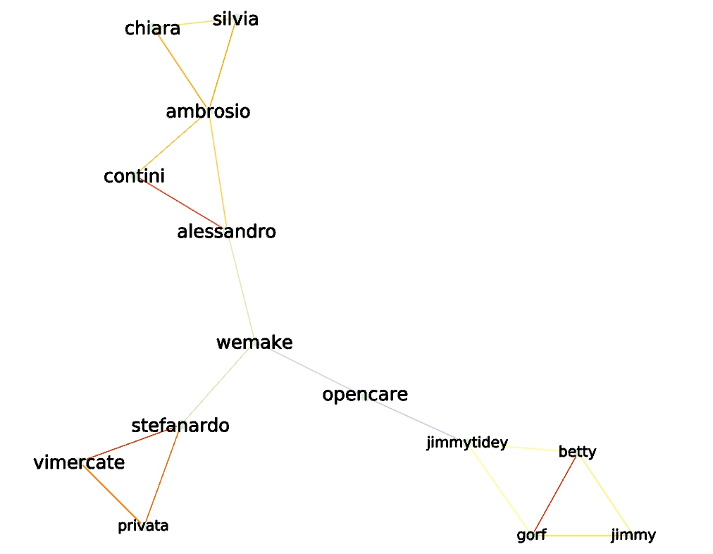
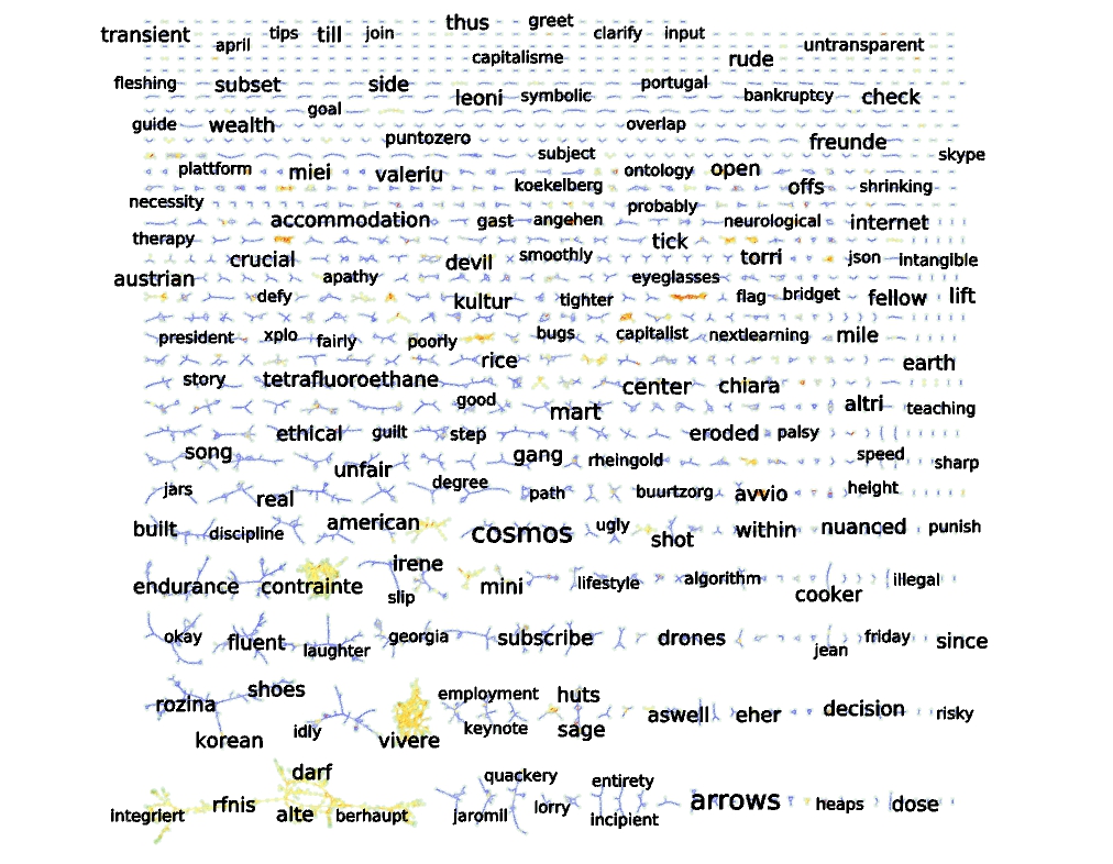
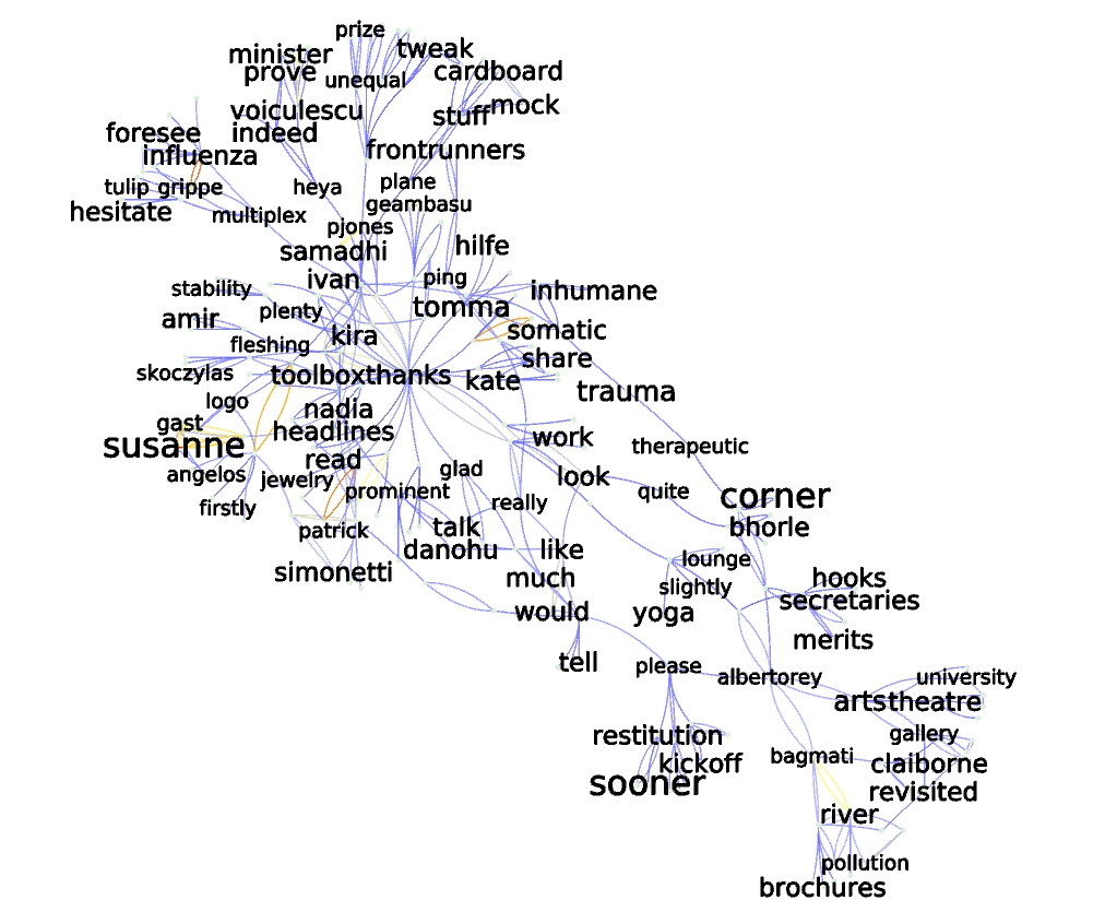
- We incremented K by step of 5 from 5 to 40, paying attention to the mutual KNN relationships. Starting from 5 the graph shows first 4 clusters corresponding to language: a bigger community for English, then Italian, French and German. When increasing K, the 4 clusters fuse rapidly to form a very dense uninformative component.
|
k=10 |
k=20 |
|
k=30 |
k=40 |


- Depending on the operations we are looking for, the choice of K is only a choice of coarse or fine filtering of the information. The graphs derived from K between 3 and 5 seem to be the easiest to tackle, but that should be confirmed only from a domain expert exploration.
|
k=2 |
k=3 |
|
k=4 |
k=5 |
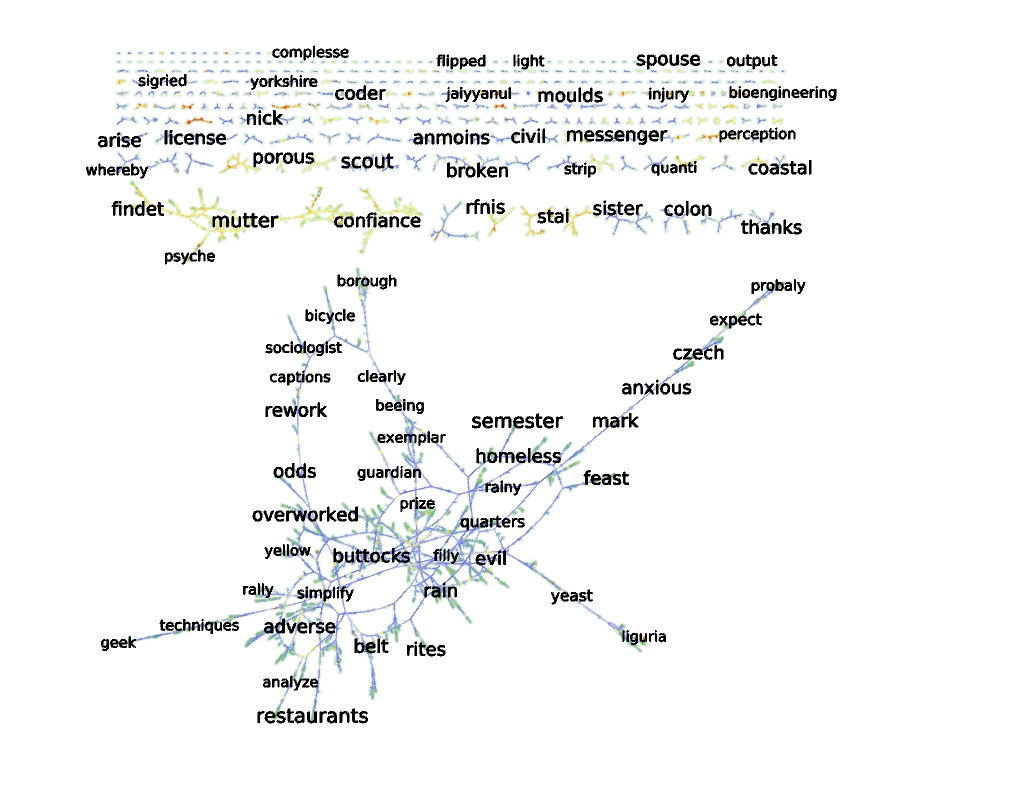


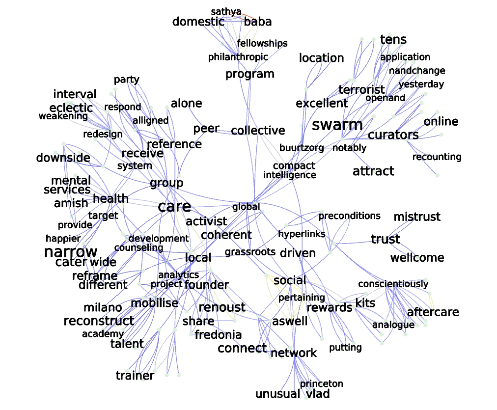
- Now the networks allow clustering the words into groups. We can try doing it either from the cosine distance or by thresholding on the euclidian distance in the layout space (e.g. after a linlog projection, since close words are supposed to be closely located on the layout).
|
Linlog thresholding |
Cosine distance clustering |

- Finally, individual neighborhood can be explored (here from reachable subgraphs with distance 3)
Query is “alberto”

Query is “noemi”

Query is “opencare”
Query is “community”
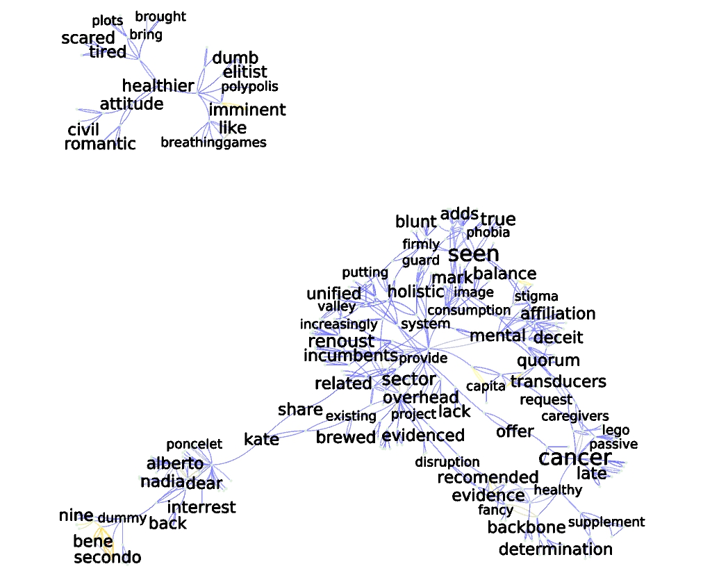
Query is “health”
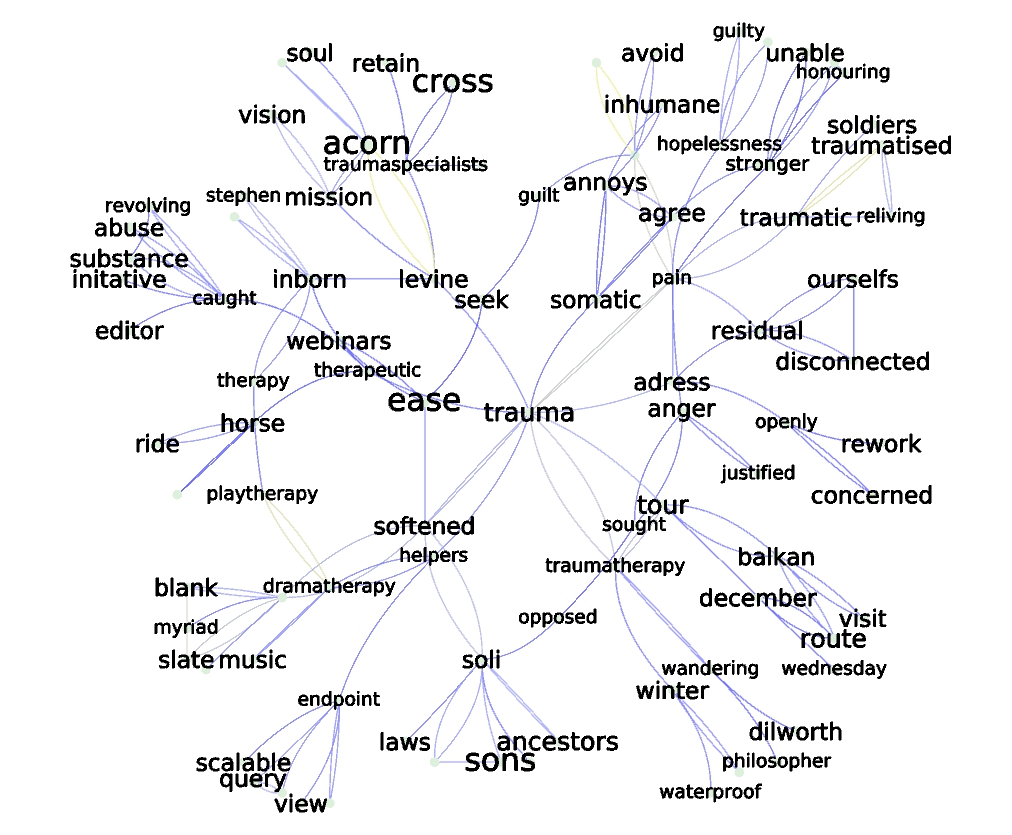
Query is “trauma”
Unfortunately the visualization was completed after the MoN5 event finished, so we can only display here the potential of the tool. The data and methods are all open, so our favorite experts are free to jump in any time.