New idea: a network approach to data saturation in ethnography?

[alberto]

This sounds a bit crazy, but hear me out. Feedback welcome. It is part of the preparations for Masters of Networks 5.

Modeling data saturation with networks

In ethnography, data saturation is the point in data collection when additional data no longer contribute to developing the aspects of a conceptual category.

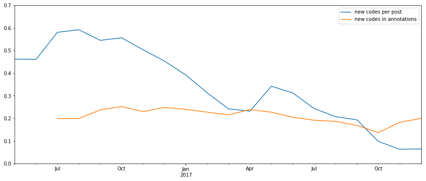
In the OpenCare project, we discovered that, as new posts got coded, they added proportionally fewer and fewer new codes to the study (blue line in the chart below). That does look like data saturation.

But what happens to data saturation when the data we are trying to discover is in network form? I refer to the codes co-occurrence network, which contains all the relevant concepts expressed as its nodes (the ethnographic codes) and their pattern of associations between them as its edges.

Let’s imagine an ethnographer who investigates a collectivity C with some research question. The answer to this question is known to C (as a collective) in the form of a network of associated concepts A, with N nodes and E weighted, undirected edges. Each edge e_A has its own weight w(e_A) (a natural number). Of course, this network is unknown to the ethnographer.

Data come to the ethnographer not in one single dump, but over time, according to a stochastic process. We can think of her accumulating data points; for example interviewing different people, who will contribute observations sequentially. Ethnography has the concept of “waves” of observation within a single study.

The ethnographer builds a model of A – let’s call it D, for “discovered” – as follows. At each step in time, she gathers a random association between two concepts in A. We can formalize this as two nodes in A, plus an edge of weight 1 connecting them. At each point in time, the probability that the ethnographer will pick edge e_A is proportional to w(e_A).

The ethnographer then proceeds to build the network D. First, she adds to it the two nodes connected by e_A, if they had not been added before. Second, she adds 1 to the weight w(e_C) of the edge e_C.

We want to show that data saturation, in this context, corresponds to the following scenario:

1. No new nodes are discovered.
2. No new edges are discovered.
3. The proportions between the weights of the edges in C are constant.

Generating a “world” to be discovered

I made a back-of-the-envelope simulation. To begin with, I built my A. The process was this:

• Generate 1,000 ethnographic codes.
• instantiate each of the possible (1,000 x 999)/2 indirected edges that could exist among them, with probability 2% (I want the network to be realistically sparse).
• Assign a weight to the about 10,000 instantiated edges. In tribute to Zipf’s Law (more on this later), I draw weights randomly from a Pareto distribution. The weight is always a natural number, so I approximate the drawn numbers to the nearest integer.
• Drop unconnected nodes.

(Python code info)

weight = 0
while weight == 0: # in rare cases, approximation makes the weight zero
weight = int(expovariate(0.2))

Simulating the discovery process in ethnography

Having generated “the world” A that we are interested in discovering, I am now ready to simulate the ethnographic observation process. Such process is divided in waves. At each wave, the ethnographer receives new information. A quantum of information is imagined to be a single dyadic association, in the form “Alice, an informant, produces a statement that associates the ethnographic codes x and y”. In other words, the ethnographer discovers edges in the codes co-occurrence network. Of course, she does not discover the weight of the edge, only that it exists. Reformulating, a quantum of information consists of two concepts, relevant to the research question at hand and representable as ethnographic codes, plus the fact that at least one informant associates them to each other. In practice, we can picture the ethnographer as drawing a random edge from an urn of edges, some of which are more represented than others.

As she discovers edges, she proceeds to add them to the discovered network D as follows:

1. Checks that the nodes incident to the drawn edges are already in the D. If they are not, add them as new nodes of D.
2. Checks that the drawn edges themselves are already in D. If they are not, add them as new edges of D, with weight equal to 1. If they are, add 1 to their weight.

To give my simulation granularity, I decided to make small waves of only 500 dyads each. This is small indeed, because a single, meaty contribution might be coded with 20 or more codes, thus instantiating a 20-clique with 20 x 19 = 380 edges.

Python code info

wave = choices(population, weights, k=sample_size)

population is a list of edge identifiers in A. weights is a list of the weights associated to each edge. sample_size is a parameter, determining how many edges the ethnographer draws in a single wave.

Simulation Results

Codes are discovered relatively quickly, edges more slowly

Within the model, it takes about 10 waves to discover 100% of the codes. The discovery of edges is much slower: even after 100 waves, 5-10% of the edges remain undiscovered.

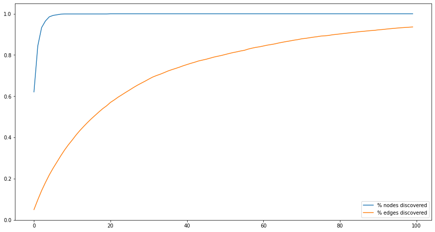
This is driven by the math. There are fewer codes than there are connecting edges (with my data, about 1,000 codes and about 10,000 edges, which is quite realistic for our SSNA studies). Every observation reveals just one edge, but two codes. This leads to a very quick ramp up of the number of codes discovered.

From the point of view of the ethnographer, who does not know the real A and so cannot compute these percentages, data saturation presents as a decline in the appearance of new nodes and edges:

High co-occurrence edges show up faster

We can argue that A also contains noise and irrelevance. Some informants will no doubt add to the data idiosyncratic connections that no one else is seeing. In empirical SSNA, we make a point of discarding all co-occurrences with weight equal to 1. What happens if we aim to discover not all of A, but only its 20% highest-weight edges? In the graph below, the green line captures the percentage of these high-weight edges discovered with each wave. After 40 waves, almost all have been discovered.

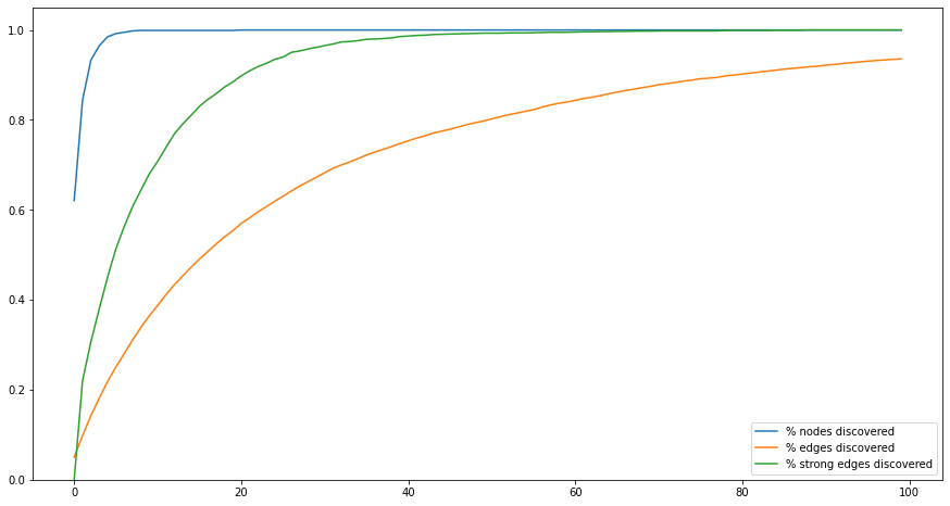
Again, this a mathematical artifact. There are fewer high-weight edges than there are edges in general, and they have higher probability to be drawn from the distribution of edges in A at each wave.

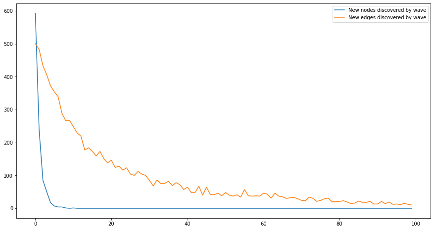
What the ethnographer sees is this:

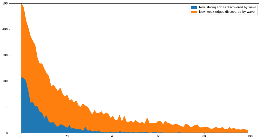
New edges appear at a slowly decreasing rate (represented by the height of the whole curve) but strong new edges (in blue) decrease much faster. Naturally, the ethnographer does not know which new edges are strong – when they first appear, they all have weight 1!

Weighing the edges

With edges, the point is not only to count them, but also to weigh them. To compare the edges of the real concept map network A with those of the discovered once D , I treat each as a vector of weights, and compute the Euclidean distance between D and A after each wave. I find it decreases at a decreasing rate. The same measure, computed for strong edges only, is lower, but does not decrease significantly faster.

Again, we observe a kind of data saturation: the reduction in distance between the discovered edges in D and the real ones in A is smaller with each successive wave. The main problem here that we have no intuitive sense of whether 0.001 distance is “pretty close” of “far off the mark”.

More on Euclidean distances

The two vectors being compared are normalized frequencies, so their distance can vary between 0 and the square root of 2. But it being close to the latter is a very rare event: it means that one of the values is 1 for one of the vectors and 0 for the other; another value is 0 for the first vector, and 1 for the second; and all the other values (about 9,998 in our case) are zero for both. This would make no sense in an ethnographic corpus: it corresponds to a network consisting of only two disconnected edges, each one connecting two of four codes in total, and they appear with identical frequency.

I guess you could have some sort of Monte Carlo method to compute a proper random-null model. Not worth getting into it at this stage.

Which distribution?

Just by how random sampling works, we know that the distribution of edges D is going to converge to the true one A. But we do not know how fast, unless we are prepared to assume a specific form of the frequency distribution of A. Recall that, in my simulation, I generated A via a Pareto distribution random number generator, but this is a bit of a shot in the dark. Not completely, though: we do know that:

1. Observed codes co-occurrence networks are generally fat-tailed. Here is a histogram of edges by co-occurrence number in POPREBEL, on a log-log scale:

   

2. Zipf’s Law tends to appear in many places. Feeble, I know…

Point is, fat-tailed distributions mean that the “important” high co-occurrence edges will be found more quickly. And in general, if we could make assumptions about about the distribution of A, then we could quantify how close we are to saturation by comparing different waves.

I could keep playing with the simulation, but best to stop here and pause for some feedback.

@amelia, @rebelethno, @nextgenethno, @melancon, @brenoust , @bpinaud … how crazy is this?