For people interested in modelling intertemporal allocation from a SF-ECON Lab perspective, there is a priceless (and simple!) article on Nature that I highly recommend: The ergodicity problem in economics by Ole Peters. The idea is to not maximize the discounted expected value of wealth, but rather “what will happen to my physical wealth as time goes by”. This is because the expected value is computed as an average of what happens to the same individual, who is taking a gamble, across multiple universes in which the gamble influencing her wealth (a random variable, a priori identical in all parallel universes) had different a posteriori realizations.
In ergodic systems, the discounted expected values (the discounted value of the realization of the random variable average across all these parallel universes) and the average over time of the individual’s wealth are the same. But most systems are not ergodic; systems in disequilibrium are almost always non-ergodic.
I will leave you to the article to enjoy the argument. For now, I want to flag to people who deal with this sort of decisions (for example in financial economics) that this might be a good way to model them.
If you are not sure whether you want to invest the time in reading the actual paper, here’s a way to get a teaser: Peters’s TEDx talk in which he explains the intuition of why human things tend not to be ergodic.
This reminded me that I actually already knew about all this, but I saw it through a different angle: in industrial economics we called it Gibrat’s law. Take a population of identical firms (or individuals, or financial assets); at each time period, let each of them grow by a rate of growth (of size for firms; wealth for individual; principal in financial assets) randomly drawn from the same normal distribution. As you let the model run, the distribution of size, or wealth, or principal approaches a log-normal distribution. A log-normal is very unequal, despite the fact that you started from identical individuals and made them grow according to the identical law of motion. Inequality is purely an artifact of randomness. Like Peters says, “everybody loses”.
Does he say if adopting one or the other average can influence choices at time t? In both cases, at a given time point, I need to make a choice with finite information (the past history/-ies).
Not sure I understand the question. Consider a bet that looks like this:
Start with 100 EUR
At each period, toss a fair coin. Heads => your money goes up 50%. Tails => your money goes down 40%.
Averaging over a large number of people playing the bet Ntimes, the value of this bet is the (traditional) expected value of its payoff, i.e. 100 x (1. 0.05)^N. Your wealth grows exponentially at a 5% rate.
Averaging over a long time, the value of this bet is -100: you lose all your wealth.
Peters uses it to explain loss aversion, currently thought to be a deviation from perfect rationality.
I have cobbled up some Python code to try it. The range of 1000, of course, can be replaced with anything. If you want a biased coin, you can enter the odds you want as an argument of the coinToss() function.
import random
def coinToss(odds=0.5):
    '''
    (float ) => bool
    returns True with probability equal to odds
    '''
    flip = random.random()
    if flip > odds:
        return True
    else:
        return False

wealth = 100
for i in range(1000):
    toss = coinToss()
    if toss == True:
        wealth += wealth * .5
    else:
        wealth -= wealth * .4
    print wealth
An interesting question is which trend is stronger. What happens when you average a large population, each member of which averages over a long time? Increasing the size of the population makes the average payoff go up; increasing the time duration of the bet makes each individual payoff go down. Which of the two trends is stronger?
I played with incorporating this code into various loops. In the end, a totally non-scientific, back-of-the-envelope test was this:
Take 10 populations of 10,000 people starting with a wealth of 1.
Make everyone play the Peters bet for N periods.
At the end of each N, count the number of people that ended up with more than 1, i.e. more than their initial endowment.
Let the model run for N = 100, then N = 1,000, then N = 10,000.
Results:
number of time periods: 100

Average of average outcomes across all populations: 42.161242451

Average number of people who increased their wealth across all
populations, normalized for population size: 0.1349

Expected value of the bet: 131.501257846
***********************
number of time periods: 1000
Average of average outcomes across all populations: 2.76743582216
Average number of people who increased their wealth across all
populations, normalized for population size: 0.00015
Expected value of the bet: 1.54631892073e+21
**********
number of time periods: 10000
Average of average outcomes across all populations: 2.42586953452e-149
Average number of people who increased their wealth across all
populations, normalized for population size: 0.0
Expected value of the bet: 7.81611065843e+211
@alberto, here’s my ergodicity econ thoughts so far . . .
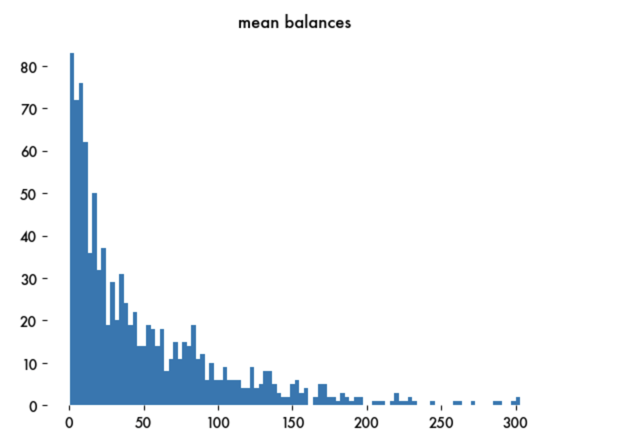
Here’s a distribution of bank account values after 100 trading steps for 1000 customers, where initial accounts are randomly populated and trading is preferential, meaning higher values accounts are more likely to trade. Note the Zipfishness.
I’m still working out how to present my Peters model results, but some observations.
Even though the initial wealth value is the same, after the first step everyone has either 150 or 60. After the second, everyone has either 225, 90 or 36, etc. So the values become spread over time. Therefore, over time the results shouldn’t change whether one is starting with a fixed or random initial value.
The Peters model is also preferential, in that the wins and loses are percent changes, so larger values will incur larger actual wins or loses than smaller values. Thus I’d expect to see Zipfiness.
The ‘gamblers ruin’ demonstrates that a random walk in one dimension will always cross a lower boundary over time. This explains while longer run lead more agents into the lower end of the distribution where because % changes yield such small results, these agents don’t move back to the 100 EU mark. (In short, this alone explains the model results to me.)
Finally, changing N from smaller to larger values is not the same as growth, which would include the endogenous addition of agents to increase N. We could try this, but I suspect system would converge to same result but over longer timeframe because you’d be constantly adding players with 100 EU. Not sure what this would imply about RW . . .
I had to read this twice to get it. It is broad way to define “preferential”, as there is nothing and no one here that prefers anything. I get it that preferential attachment => power law, so the distributions are related at least, but if I were a layman the term would confuse the hell out of me.
Yes, I agree it is confusing, but the effect is the same. Your Gibrat example is closer, large cities and small cities ‘grow’ differently as a direct function of their size, and it’s the size effect that matters, though concepts like preferential attachment or preferential trading are also size determined. I don’t know of a succinct term for that.
… although Gibrat’s law starts from empirical observation, not mathematical modeling. That is, the distribution reflects also creation and dissolution of companies, rather than the fixed-population toy world of the Peters model.