Will your mini-presentation be a document or are you presenting it live? If the latter, can you send a Zoom link?
Where are we?
Dear All, I suppose something came up and the meeting was cancelled. I am going to start inserting my suggestion to the draft over the next 4 days, but I need a “privilege” of an editor. The system tells me I do not have it. Ciao.
Document. We were not ready to give it today.
No, it was just that I needed to get together with Guy and Bruno to discuss some technicalities and assign homework.
You are going to need this link.
To-do list for the computation group:
- @bpinaud: re-run the scripts for computing network reduction based on association depth and association breadth on the fresh data export. I sent it to you yesterday.
- Bruno and Guy: compute network reduction based on Simmelian backbone. As link strength we have decided to use association depth, but see my next post below.
- @melancon: based on the literature, provide the maximum number of nodes and maximum density for a graph to be still visually interpretable. This goes in section 5.1.
- Based on these parameters, Bruno computes the maximal interpretable reduced network for each method. We can then compute a matrix of Jaccard coefficients of the codes and edges for each pair of reduced networks, and that becomes a cornerstone of our final results.
- Bruno: can you also take care of plots? I am superbad at it, and it takes me forever to make them. Yet, I feel that we should use plots rather than tables, to be friendlier to the intended audience.
For all co-authors, but especially @bpinaud and @melancon: I completed the data crunching on k-cores as a reduction method, and here are my thoughts.
TL;dr: I don’t think k-core decomposition is a very effective method for network reduction. It is difficult to tune, difficult to interpret, vulnerable to outliers (single posts with many codes). Furthermore, by construction it leads to high-density reduced networks, whose topological information is difficult to interpret visually.
“Pure k-core” method
The main idea is that important edges (the ones we want to keep when reducing the network) are those that connect two highly connected nodes. Since we are doing network reduction, and not community identification, I proceeded as follow:
- For each node, compute the core value (the maximal k for which the node is part of a k-core). I chose to treat the graph as unweighted, to make it a “pure topology-based” reduction method.
- Start at
k = 1. Drop all the nodes for whichk < 1. Count the remaining nodes and edges. - Then do the same for
k = 2, and so on.
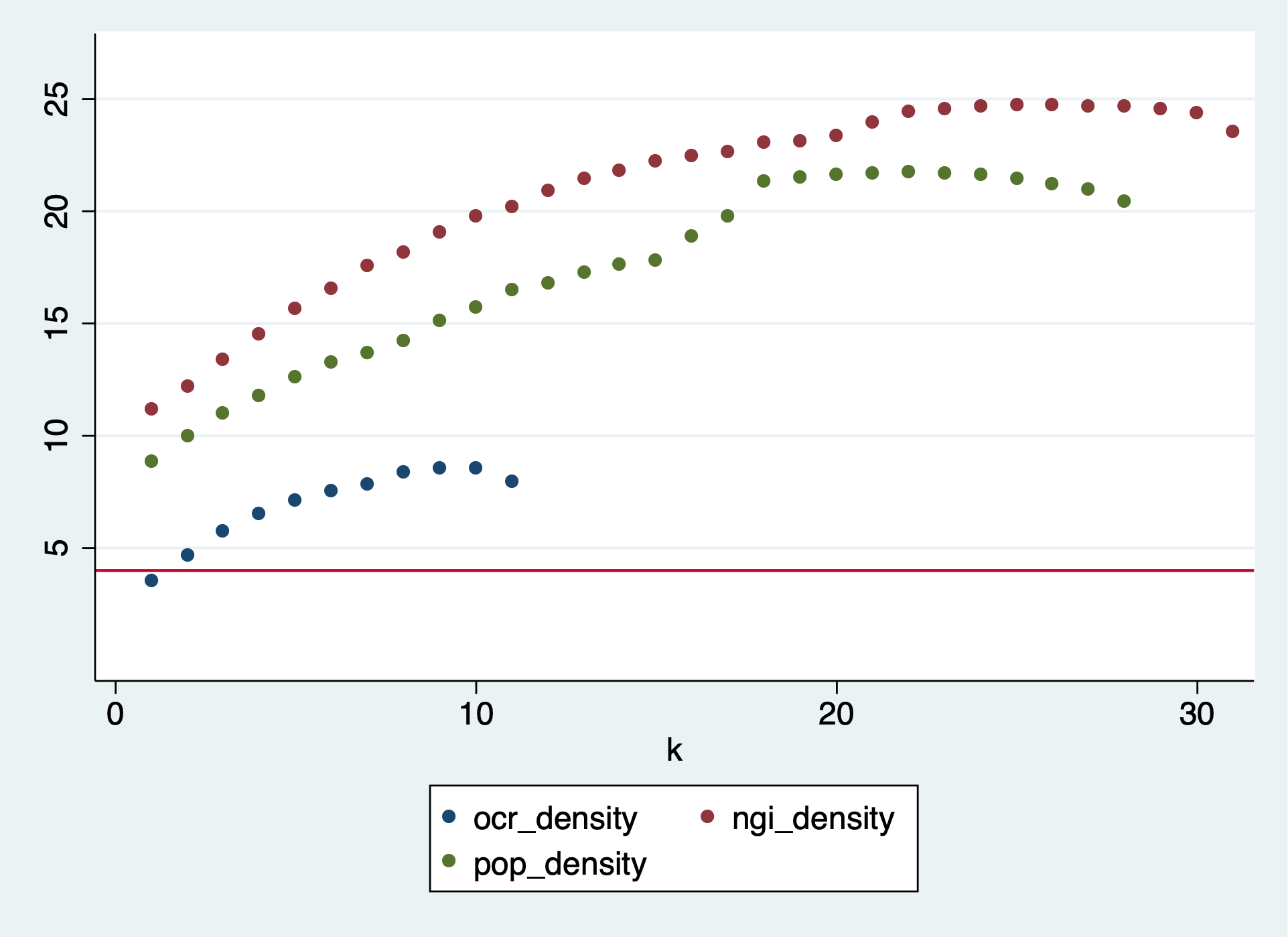
Results (normalized for comparability):
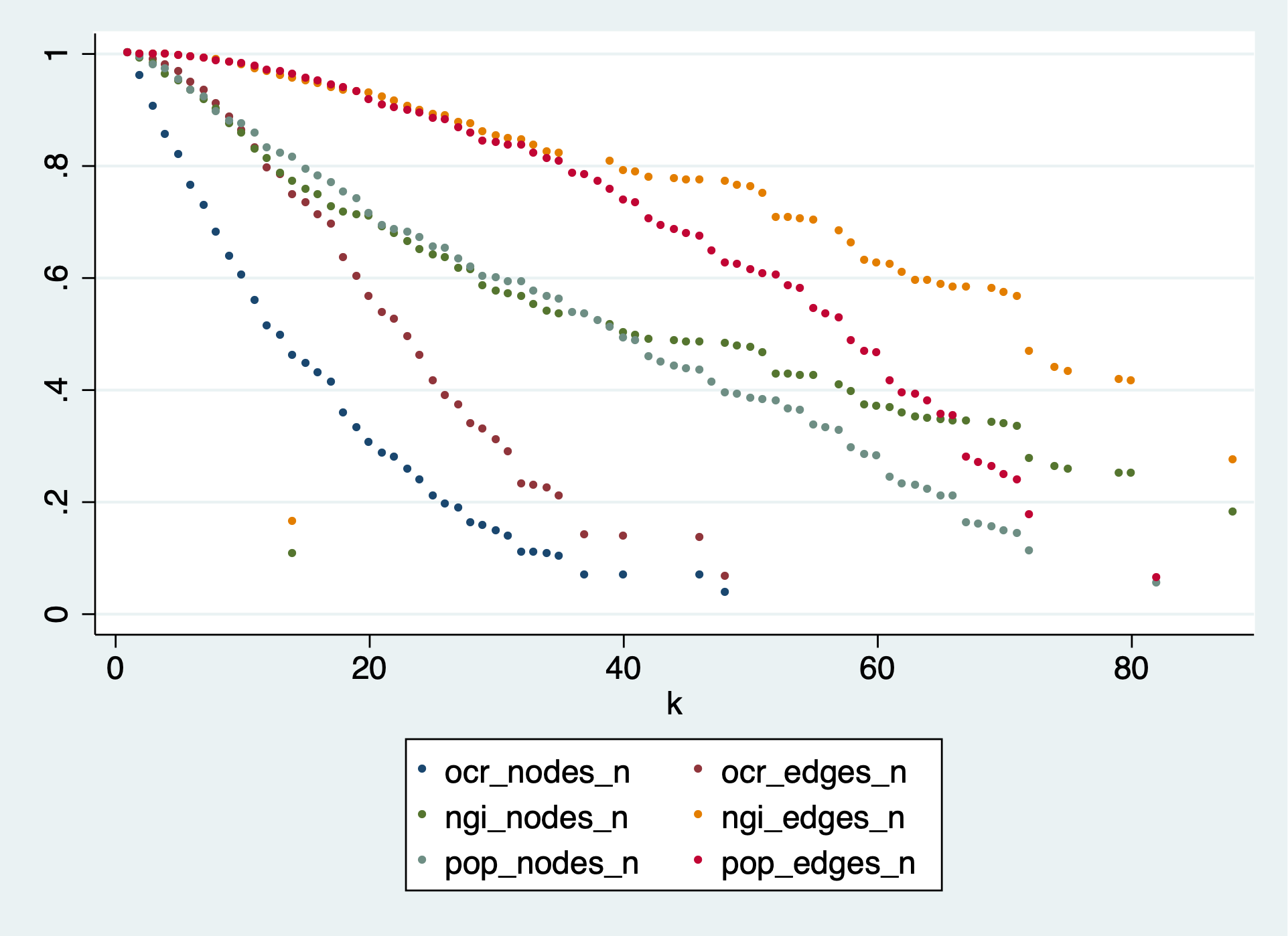
Reducing the graph by dropping low-k nodes is slow going – just compare that with the figures in sections 5.2 and 5.3 of the paper. This is logical, because we start dropping the least connected nodes, and keep all the hubs, who have lots of edges. Even at the highest possible value of k the POPREBEL reduced network has 83 nodes and 3,403 edges.
This is confirmed by looking at how edge density changes in the reduction process: it increases instead of decreasing. None of the datasets comes even close to crossing the line of 4 edges per node that would make the graph readable.

But there is an even more serious problem: I re-read the Giatsidis et al. paper, and, sure enough, they manually drop very high-k nodes from their dataset. Their case is networks of co-authorship of academic papers: the dataset included a paper with 115 authors. This made every author of that paper look like they were more degree-central than Paul Erdos! With us, it is the same: a single post with lots of codes gives rise to a large clique, and so it dominates the result. Collective intelligence is lost, what you are seeing is mostly the longest, most interesting post in the corpus.
From this kind of consideration, Giatsidis derives the idea to normalize to 1 the maximum co-authorship value for each paper. In that case, an edge deriving from the 115 authors paper has weight `1/(115*114) =~ 0.00007. We could do that, of course, but that has another problem: you end up with very many different values of k, and the cores are very small.
The most densely connected core (k = 82) we are left with at the end of the reduction in the POPREBEL corpus has 83 nodes and 3,403 edges, with a density of 40 edges per node. The graph is just a gigantic hairball. Here are the codes, in case @Richard, @jan or @amelia have an intuition:
upside of COVID
family structures
vaccinations
EU
political marketing
Media
religion
atheism
religious upbringing
traditional values
Catholic Church
LGBT
Andrzej Duda
mudslinging
prohibition of abortion
Civic Platform/Coalition
discrimination
populism
Law and Justice party
personal liberty
unemployment
closures
pandemic
seeking civilised debate
health expenses coverage
need of a third option
polarisation
separation of Church and state
evidence based
state funds mismanagement
entrepreneurs
political self-interest
Polish catholicism
provinciality
anti-clericalism
informal social support
Warsaw
Arts and Humanities
*fear
belonging
*sense of safety
trust
mental issues
Youtube
politicisation
construction of common identity
left wing
imagining the future
alienation
engagement
‘Polishness’
sense of increase
civic awareness
learning languages
‘global citizen’
Ukrainians
freedom of movement
foreign-language press
Gazeta Wyborcza
newspapers
military conflict
revolution
“the Jews”
respect
constitutional court
political choice nobody
therapy
welfare state
exclusion of straight white males
unity
votes buying
pluralism
eye for an eye
empathy
homophobia
xenophobia
political changes
k-core method applied to a pre-reduced graph.
I tried a different approach: delete all edges with association breadth = 1, then apply reduction as described above. The results are similar, but starting from an already much smaller and less dense graph:
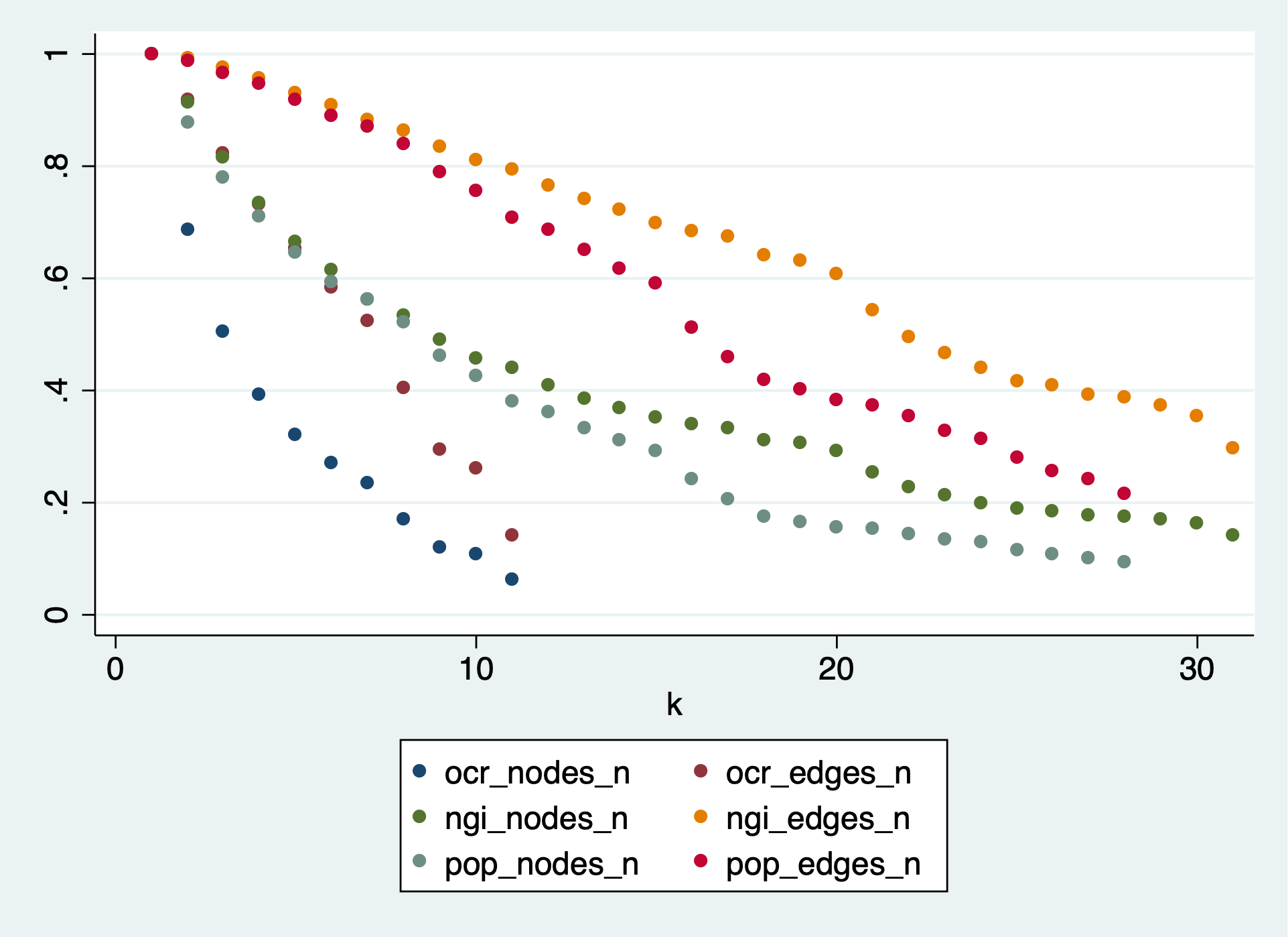
In the POPREBEL corpus, the highest-k nodes are connected in a core with 70 nodes and 1,429 edges. At 20 edges per node, the graph is just a hairball. The list of codes is:
family structures
freedom
education system
inadequate income
Media
religion
atheism
religious upbringing
traditional values
corruption
Catholic Church
tolerance
LGBT
(lack of) affordable housing
big cities
‘right wing’
political activism
disappointment
Civic Platform/Coalition
discrimination
Law and Justice party
political choice right
unemployment
seeking civilised debate
polarisation
separation of Church and state
estranged authorities
entrepreneurs
abuse of power
nationalism
provinciality
democratic elections
low quality of the health care system
informal social support
*fear
dogmatism
lack of solidarity
despondency
mental issues
conservatism
politicisation
construction of common identity
left wing
alienation
‘Polishness’
sense of increase
Ukrainians
welfare state
pluralism
xenophobia
Germany
democratic backsliding
political inaction
cities
mass media
polarisation political
universities
social benefits
inequality
sense of agency
lack of support
religiosity
neoliberalism
need for change
draw of populism
social activism
manipulation
hate
social sensitivity
polarisation cultural
Conclusions
I think we should not recommend this method of network reduction. We could still present it in the paper, or relegate it to an appendix, but it is not good. Because:
- Slow and unwieldy – the only way to get the number of nodes down is to use the very highest values of
k. - More difficult to interpret mathematically than simple link strength.
- Vulnerable to outliers (long posts with lots of codes that tend to dominate). There are remedies for that, but they mean combining various methods, and that makes interpretation more difficult and diminishes research accountability.
- By construction, it keeps highly connected nodes, so the reduced networks are very dense.
In general, reducing CCNs based on measures of link strength seems a superior strategy.
1 Like
Hi all,
just to give you an update of what Bruno (@bpinaud) and I have been looking at today during our working session. The overall plan was to:
- have a look at numerical figures to compare the different methods (ongoing)
- compute network reduction using the so-called Simmelian backbone approach by Bobo Nick
I want to report here on the second item. First I need to provide a bit of background so you get what the method does: how it proceeds to filter out edges. The main idea follows a quite classical schema: you compute a statistic on edges, called edge redundancy, and skim out edges with low redundancy to only keep those with higher redundancy, with the rationale that higher redundancy leverages edges that form the backbone of the network.
Redundancy is easily defined: an edge is redundant if it is part of multiple triads (this is why the authors named the method after Simmel). Recall that an edge is part of a triangle exactly when its endpoint have a common neighbor. So triangles containing an edge coincide with common neighbors of those nodes incident to that edge.
Now, Bobo Nick adds a little spice to the method. We assume we have a criteria to assert than an edge is strong, that is we can say when an edge e is stronger than an edge e’. For that, we can use the number of co-occurrences attached to the edges. We also need to fix a parameter k: we will only look for triangles formed using the k strongest edges.
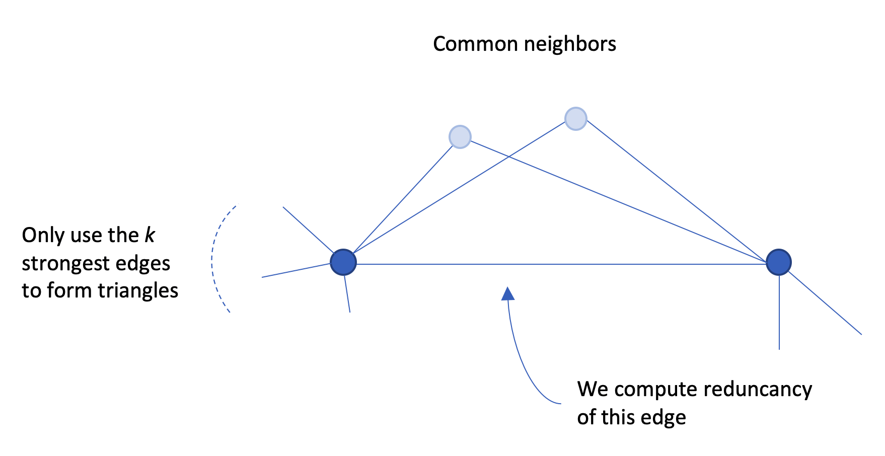
We observed, with the network data we have, that nodes have on average a degree of about 20 (tags
connect to 20 other tags). Hence, our intuition guided us to experiment the method using k = 20.
–
Question for you all: is there a more domain related rationale for choosing a value for k?
–
Recall, that the result of the preceding steps results in assigning each edge a redundancy value r. The network can then be skimmed from its low redundancy edges to produce more readable images, leading from a classical hairball (1391 nodes / 17364):
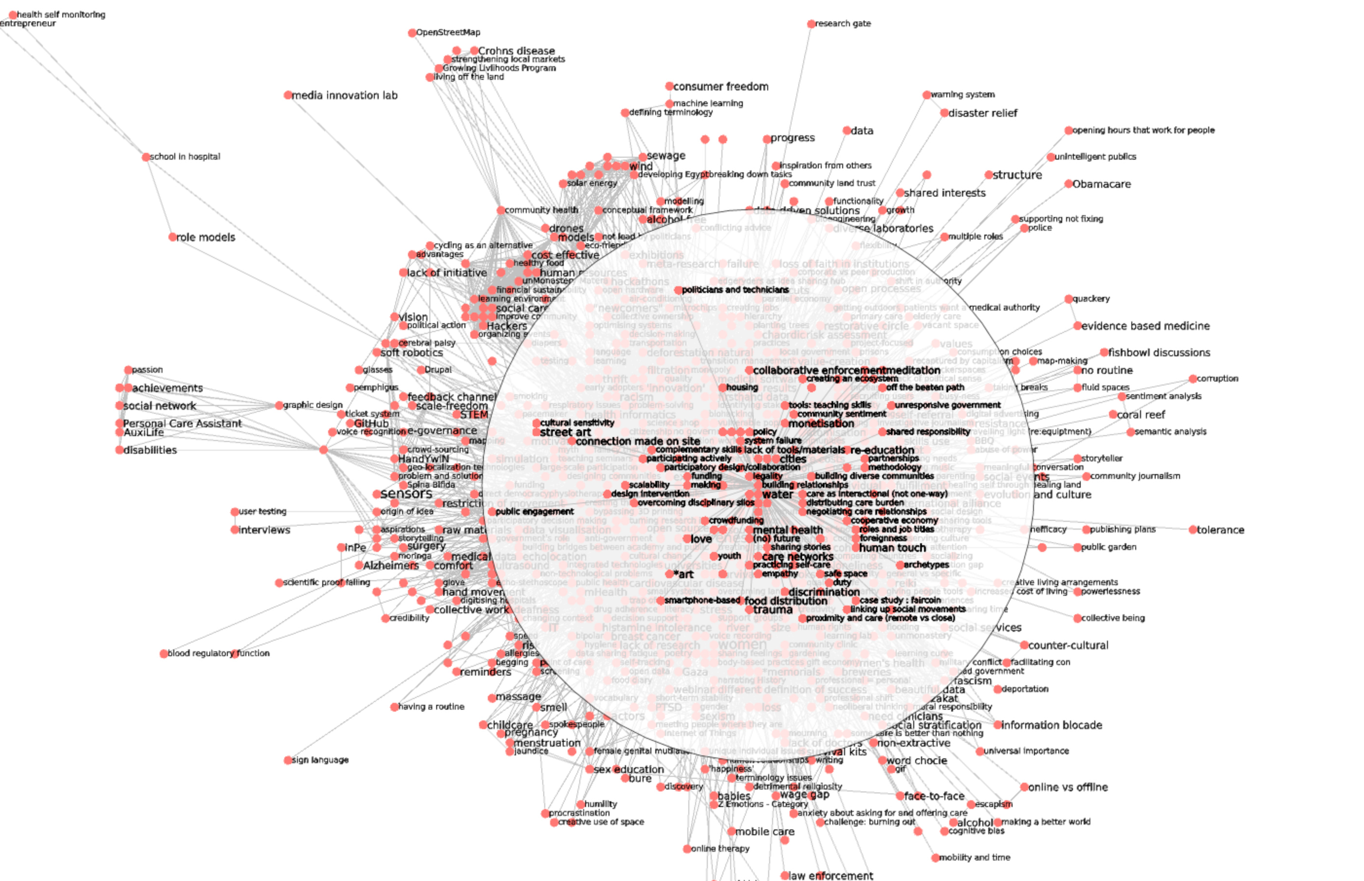
to a less dense network (510 nodes / 4275 edges when discarding edges with redundancy less than 15, together with isolated nodes):
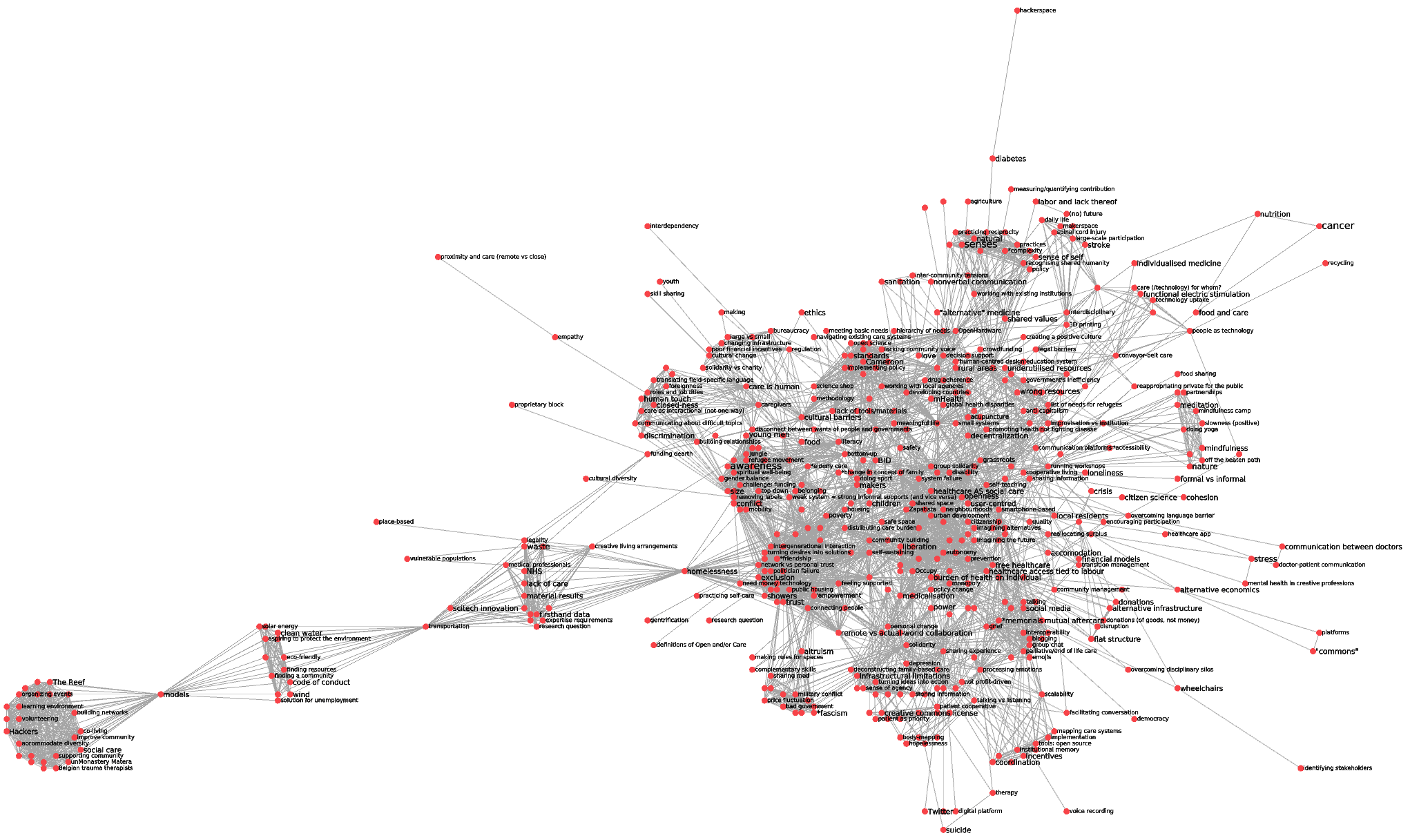
To mimick @alberto’s reasoning, I have extracted the tags attached to edges in this reduced network. Collecting tags from the 500 strongest edges, I get (by alphabetical order):
‘empowerment’
“boxpeople”
*friendship
alternative infrastructure
anti-racist
atomisation
burden of health on individual
burnout
colonisation by medical profession
commodifying bodies
connecting people
coworking space
definition of community
difficulties
distributing care burden
exclusion
feeling supported
free healthcare
happiness vs fitting in
healthcare access tied to labour
healthcare AS social care
individual
lack of knowledge/skills
liberation
maintaining social networks
makers
medicalisation
network vs personal trust
NGOs
Occupy
political groups
politician failure
poverty
public housing
public-private partnerships
redefining health
remote vs actual-world collaboration
removing labels
self-selection
self-sustaining
shared space
showers
social care (soft) vs medical care (hard)
systems-based vs family-based care
technology
treating people like adults
trust
turning desires into solutions
understanding own body
using existing infrastructure
visibility
working with policy makers
Zapatista
–
We still need to pursue our work. Hope what I have posted makes sense anyway.
1 Like
Not a surprise, we worked on the OpenCare dataset
Ah! Thanks Bruno, I forgot to mention this …
Great work!
I doubt it. What you can do is work in reverse: start from a desired “amount of reduction” that will make the network readable, and then choose the values of the parameters to obtain that amount. I used that reasoning here.
Your reduced network is much larger than the ones I computed (I am around 200 nodes, 600 edges). But your reduces network is somehow fairly legible anyway. I think this is the added value of the Simmelian backbone method. I seem to recall, from reading Nick’s thesis, that his method led to highly modular networks, and again what you obtain here is very modular. This mitigates the readability problems associated with high network density – and indeed your reduced network, while very dense (dl = 0.16 using Ghoniem’s measure of density), are still readable, at least to me. What do you think of this, @amelia, @jan and @richard?
Then, an analytical strategy available to the qual researcher is to examine each codes community separately (and they are nice and small, 10-40 codes each approximately). She could even wrap each community into a metanode and look at the resulting network of metanodes – I imagine there would be between 15 and 20 of those. This is a result, congratulations!
Hmm… we need to agree on a way to compare the reduced networks. I was thinking of Jaccard coefficients on the entire list of nodes, but that works best if the reduced networks are approximately the same size, which they now are not. @bpinaud, you were going to compute these statistics… any idea?
We also work on Jaccard index and other measures with Guy.
Here is my understanding of what to do:
Data: for each of the three data sets and for each of the four reduction methods, we have a series of graphs (10 to 12) starting from the complete stacked graph to a very reduced readable and legible graph (around 200 nodes and 600 edges).
Aim: for the most reduced interesting graphs (instead of what i did to generate the IC2S2 reduction document on google drive) we can check if the edges are the same/almost the same between the four methods and for each datasets. We can simply compute the ratio of common edges between each graph (easy to do with Tulip). Of course, we have to plot the reduction behavior of nodes/edges for each method and each graph.
My questions: do we need to compare the graphs (ratio of common edges) at each step of the reduction process?
In the end, the Jaccard index cannot be used because the sets to compare must have the same number of elements. We think that the ratio of common edges between two graphs is enough.
1 Like
Almost. For more rigor, I would like to set the size of the reduced network in ways that are supported by the netviz literature. But I am super ignorant around that. I tried to rummage into Google Scholar, but was completely unsuccessful. So I am stuck with Ghoniem 2004. His largest graph, that is still low-density enough to be understood by the people interpreting it in his experiment, has 100 nodes and dl = 0.2. Now, dl is dependent on network size, like Guy famously observed. A network with 200 nodes and 800 edges (Guy’s “four edges per node” rule of thumb) has dl = 0.18. This is how I landed on “no more than 4 edges per node, dl < 0.2”.
But this is pretty weak. Do you guys have any pointers to more recent work on how large and dense networks can be for humans to still be able to make sense of them?
In theory, no. Because the reduction process stops at a point that has nothing to do with the ratio of common edges, but only with the visual processability of the reduced network.
Why? You can certainly compute the index (number of elements in (A intersection B)) / (number of elements in (A union B)) for any number of elements in A and B. Of course, it those numbers are different, that number can never be 1. But you could solve this by rescaling for the maximum possible value attainable by the coefficient J.
For example, imagine that set A has 10 elements and set B has 5. The maximum value attainable by J is 0.5, in the case that all 5 elements of B are also in A. In that case, A union B has 10 elements, and A intersection B has 5, so 5/10 = 0.5. Now rescale this to 1, and rescale the actual value of the Jaccard index accordingly. For example, if 3 elements of B were also in A, you would have:
- A union B has 12 elements
- A intersection B has 3 elements
- *J(A,B) = 0.25 => rescaled it becomes 0.5.
Ok, but what is the denominator here?
Hi all! @Jan, @Richard and I just had our meeting and wanted to ask if you all would be able to give us 2-3 different reduction approaches to the POPREBEL dataset so we could better answer some of your questions based upon the data we know and are familiar with. In the meantime we are getting down to writing!
Not sure I understand the question… the paper is going to contain four approaches. Two – by association depth and association breadth – are already explained in the Overleaf document. An application to the POPREBEL dataset is here, though complicated by the languages issue.
The other two are: by k-core decomposition, applied to POPREBEL here; and Guy’s Simmelian backbone, applied to POPREBEL data here.
What would you need exactly?
@alberto - many thanks. We will study this and get back to you if we have questions (most likely we will have - we are working to bridge to qual-quant divide, after all ![]() ). For now we are creating a separate google doc to work on our (@amelia and @Richard) contributions to the opening part of the paper. It is here.
). For now we are creating a separate google doc to work on our (@amelia and @Richard) contributions to the opening part of the paper. It is here.
1 Like
Obviously yes. However, I am pretty sure, that we can find a better similarity measure between 4 sets of different sizes
Ok, now I am confused. “Stronger” edges means edges with a high association depth d(e). That has no bearing on the degree of nodes. Why do you use average node degree to calibrate k? Also ping @bpinaud.
We used the degree because it is a standard and basic measure (the higher the degree, the higher chance of having the node involved in more triangles). k relates to connectivity (see Guy’s previous post on the definition of k).
1 Like
Noted.
Ok, but
SInce k = 20, this sentence becomes “we will only look for triangles formed using the 20 strongest edges”, which is clearly not the case!